by Rick O'Connor | May 20, 2022
Imagine…
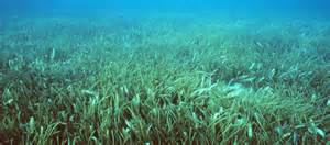
It is 1922 and you are rowing your wooden skiff from a small beach house near what will become the town of Gulf Breeze Florida across Santa Rosa Sound on your way to Santa Rosa Island. The water is 10-15 feet deep, and you can see the bottom. It is covered with a lush garden of seagrasses with numerous silver fish jutting in and out of the blades. Most are there only for a moment before they are lost again. You notice a brown colored puffer fish hovering over the grass as you past by. Maybe a small sea turtle grazing, or a tannish colored stingray flying over the meadow. As you get closer to the island, which is covered with sand dunes reaching 20-40 feet in height and shrubby live oak and magnolia trees, you begin to see Florida conchs and horseshoe crabs, maybe fields of bay scallops littering the grass in every direction.
An amazing meadow of underwater grass.
Photo: Virginia Sea Grant
Sounds amazing, doesn’t it? And it was actually like this once.
What changed?
I asked this question of some ole timers who grew up on Bayou Texar in Pensacola decades ago. You might be surprised to learn that Bayou Texar resembled this scene. They described water that was between 10-15 feet deep, had sand and seagrass on the bottom, and you could catch shrimp the size of your hand by tossing out a cast net. But Bayou Texar no longer looks like this.
Most told me the first thing they remember was a change in the water clarity. The water became more and more turbid. Then the shrimp went away, then some of the fish. They mentioned several species of fish that no longer exist there. The cause of the turbid water? … Development. They were developing all around the Bayou after World War II and that was when things began to change. They mentioned the road going in on the east side of the bayou as the point when turbidity issues began. The houses came later.
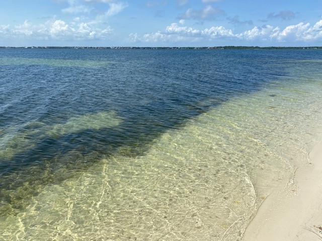
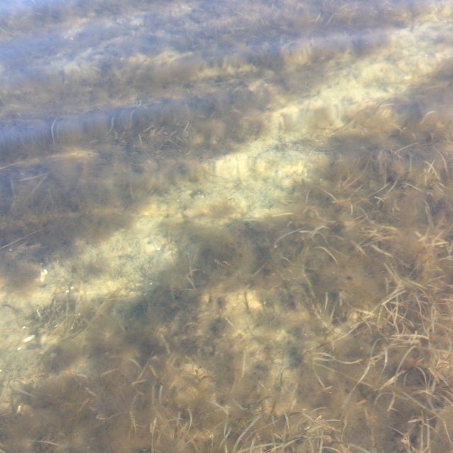
With little rain over the last few days the water clarity was excellent and you could see the seagrass very well.
The city of Gulf Breeze was founded in 1935 and was originally called Casablanca because of a white house there that could be seen from Pensacola. As the community grew the waters became more turbid as well, and the amazing underwater garden declined. But this was not just happening in Gulf Breeze and Bayou Texar, it was happening everywhere.
But it was bound to happen. As the human population grows more space is needed for homes, businesses, and schools. More roads are needed to reach these locations and a bridge was placed to reach Santa Rosa Island, so you no longer had to paddle a skiff to reach it. Once on the island, growth continued. More homes, roads, and businesses. With more run-off, turbidity, and the garden continued to decline.
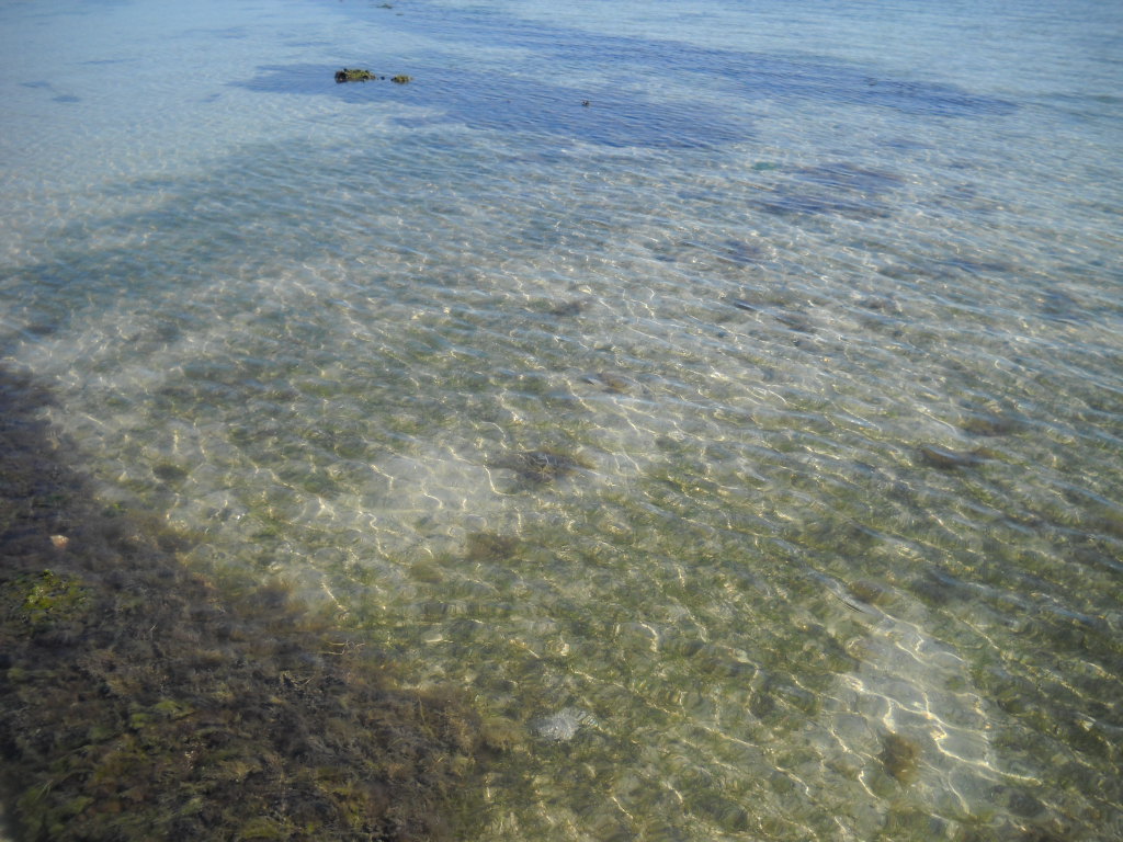
Shoal grass. One of the common seagrasses in Florida.
Photo: Leroy Creswell
The thing was we did not know at the time that (a) we were causing this decline and (b) how much we really wanted that garden there. I often hear the question “what happened to all of the blue crabs?” I think they know the answer, but they remember a time when blue crabs were more abundant, can you imagine what it probably was like for our friend paddling across in 1922. And there has been a noticeable difference in crab numbers in their life. There are folks, including myself, who remember bay scallops in the Sound and horseshoe crabs on what they called “Horseshoe Crab Island” in Little Sabine. This is one of the amazing things about this story – how fast the decline was. Now we better understand how important these underwater meadows were to the function of a healthy estuary and there is interest in restoring them.
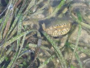
Bay scallops need turtle grass to survive.
Photo: UF IFAS
To restore seagrass, you first have to understand, and mitigate, what is causing the decline. Seagrasses are vascular plants that possess roots, stems, and leaves. They produce flowers and sexually reproduce using seed. This is not the case with seaweeds, which are nonvascular and lack the above, but they often mistakenly called seaweeds. There are three species that dominate our seagrass meadows in the Florida panhandle and a fourth one that is not as common. The uncommon one has a round blade like a pine needle and is called manatee grass (Syringodium filiforme).
The three common species all have flat blades. Widgeon grass (Ruppia maritima) has blades that branch. It tolerates a wide range of salinity and is more abundant in the upper regions of our estuaries. Shoal grass (Halodule wrightii) has a single flat, non-branching, blade that is very narrow (< 3mm) and resembles human hair. Turtle grass (Thalassia testudinum) is also flat, non-branching, but wide (>3mm) and resembles St. Augustine grass.
Like other grasses, these plants require sunlight and nutrients to survive. They also need to grow in the low energy locations of our estuaries. Sunlight, of course, is key for photosynthesis and clear water is the key to getting enough of it. 15-25% of the sunlight reaching the surface of the water must also reach the bottom where the grasses are. Nutrients can be obtained through the water column and sediments. The stems run horizontal beneath the sand and are called rhizomes. They help hold sediments in place increasing the much-needed water clarity as well as reduce shoreline erosion. The blades extend from the substrate up into the water column bathing in the sunlight. They are covered by microscopic plants and animals that resemble scum when you run fingers over them but provide mush of the food for the creatures that live there.
And live there they do.
It has been estimated that it least 80% of the commercial and recreational important shell and finfish spend at least part of their lives in the seagrass meadows. Ducks, manatees, and sea turtles are some of the grazers on these plants and sea horses, pipefish, and pinfish are abundant.
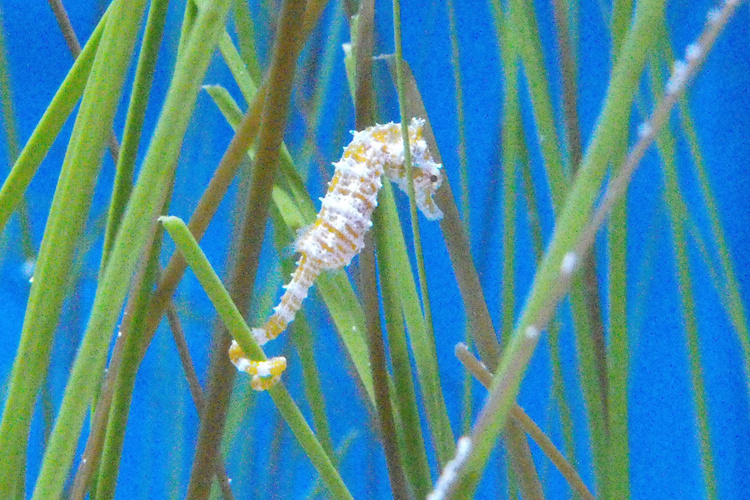
Photo: NOAA
When humans began developing around the Sound in the 1940s and 1950s the sediment run-off decreased water clarity, cutting off the much-needed sunlight, and in some locations covered the grasses. Excessive nutrients from our fertilizers, and detergents increased phytoplankton growth which in turn decreased water clarity more and enhanced the growth of macroalgae which smothered the meadow like a blanket. Hot water discharges from industrial processing along the shores stressed the grasses as did prop and anchor scars from power boat plowing through and anchoring in them. These same boats and jet skis increase wave energy with their wake, as do seawalls when waves reflect off of them. Marinas, bridges, and docks all required dredging in the meadow which not only removed the grasses but increased turbidity even further. All of this triggered the decline of these amazing gardens. And with them the decline of the cherished fisheries as well.
The scarring of seagrass but a propeller.
In recent years the Florida Fish and Wildlife Conservation Commission (FWC) conducted surveys across the state to assess the status of our seagrass beds. They estimated that there was a little over 2 million acres of seagrasses in Florida waters, 39,000 in the western panhandle. Though much of these beds appeared to be stable, or even increasing acreage, those in the panhandle were still in decline and all of Florida’s seagrass gardens were less than the acreage in the 1950s.
In this study they found the Perdido Bay had primarily shoal grass. Big Lagoon and Santa Rosa Sound were a mix of shoal and turtle grass, with some manatee grass reported from Santa Rosa Sound. Aerial imagery found –
Perdido Bay had 642 acres of seagrass in 1987; 125 acres in 2002 for a net loss of 5.4% / year
Pensacola Bay had 892 acres in 1992; 511 acres in 2003 for a net loss of 3.9% / year
Big Lagoon had 538 acres in 1992; 544 acres in 2003 for a net gain of 0.1% / year
Santa Rosa Sound had 2,760 acres in 1992; 3,032 acres in 2003 for a net gain of 0.9% / year
The numbers in the lower portion of the bay are encouraging and suggest some behavior changes we made in recent decades have helped. Both development and monitoring continue. We will see.
What can be done to help restore the garden?
- First, reduce run-off into the bay. This can be done by engineering designs with green infrastructure methods but can also be done by the private homeowner as well. Using native plants in your landscape reduces the need to irrigate your property and landscape designs which include rain gardens and rain barrels will also help reduce run-off.
- The reduction of nutrients begins with the reduction of fertilizers on the landscape. Using Florida Friendly Landscaping principals can lead to a beautiful landscape that does not require fertilizers. If you choose to use nonnative plants that do require fertilizers, use only what the plant needs – do not over do it.
- If you live along the waterfront, you can further reduce nutrients by planting a living shoreline. The plants used in living shorelines are known to remove nutrients from run-off from your property, as well as reduce erosion and provide more habitat for fisheries. One living shoreline project in Bayou Grande has seen an increase in shoal grass beds since they planted it.
- When boating, be aware where seagrasses exist. Lift your motor when moving through them to avoid prop scarring and anchor in open sandy locations. You can also follow the principals of a Florida Clean Boater to reduce your impact on water quality that could impact the seagrasses.
With a little effort on our part, we can enhance some of the positive numbers we have seen in seagrass assessments and hopefully turn the current negative trends into positives. Maybe the garden will return. For more information on how you can apply any of these principals contact your county Extension office.
by Rick O'Connor | May 13, 2022
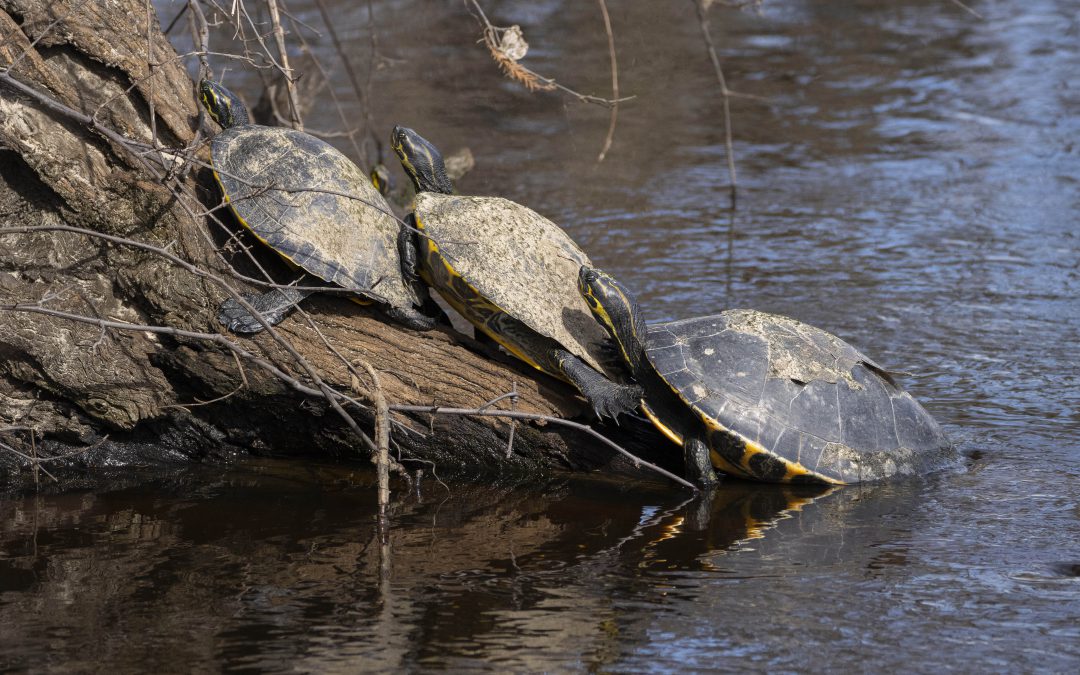
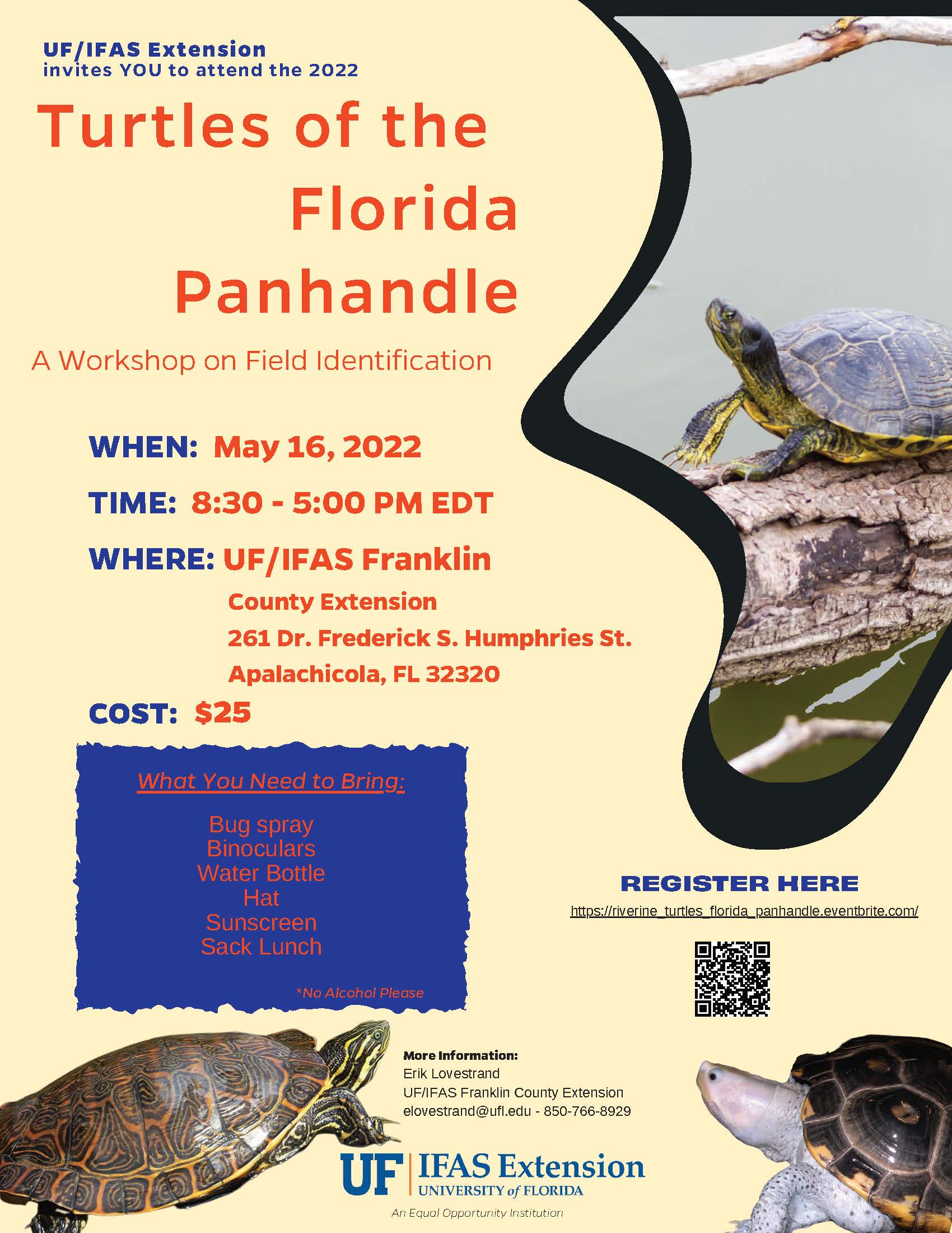
The Florida panhandle has one of rich biodiversity. This goes for the variety of turtles found here as well. Many paddlers and hikers to our waterways see these turtles but have trouble identifying which they are looking. In response to request by outdoor adventures wanting to learn more, UF IFAS Extension will be offering a one day workshop on field identification of panhandle riverine turtles.
The workshop will be held this Monday – May 16, 2022 – in Apalachicola FL. Participants will attend a classroom session where the biogeography of our turtles will be discussed and visual identification will be practiced. We will then take a boat ride up the Apalachicola River and practice in the field.
The program will begin at 8:30am (ET) at the Franklin County Extension Office. The cost will be $25 and preregistration is required. You can register at https://riverine_turtles_florida_panhandle.eventbrite.com/
by Rick O'Connor | May 13, 2022
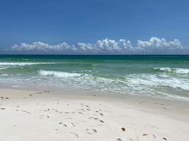
It is mid-spring and time of nesting for much of the wildlife in the area. It is also noticeably warmer than our previous hikes. Due to my work schedule, and the surveys for other nesting activity, I did this hike earlier in the month and later in the day, than I typically would have. I began my hike at 1:00pm – near the hottest part of the day, and not the best time to see wildlife, but I definitely wanted to get a hike in this month and so this is when I could.
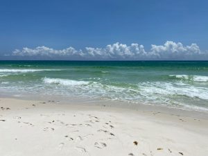
The Gulf was relatively calm on this early afternoon in spring.
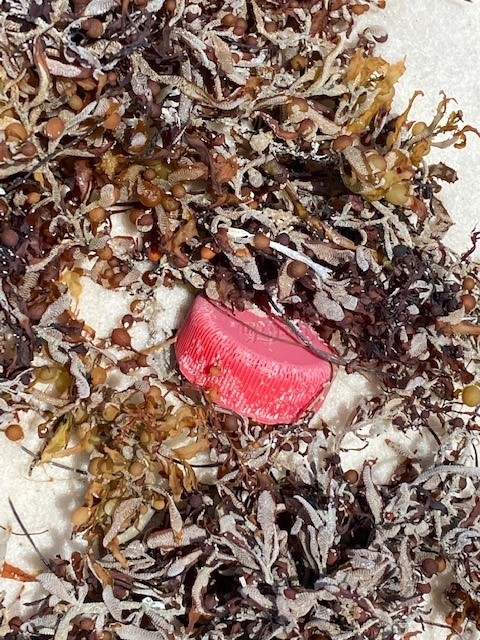
It was warm. On this day it was 83°F and there was a light breeze from the southeast. On the previous hikes I needed my fleece. Though I had it in my backpack, I did not need it today. My hike was at Big Sabine and as usual, I began on the Gulf of Mexico. The first thing I noticed when I crossed over the boardwalk was the number of people. I usually hike in the early morning or late afternoon and see few humans. But at mid-day the beach was full of people, and I probably looked strange walking among them with my long pants, long sleeved shirt, and boots. The second thing I noticed was mats of Sargassum on the beach.
Sargassum is a floating brown algae we see in the warmer months in our part of the Gulf. It is first an algae, not a true plant. Algae lack roots, stems, and leaves. They produce no cones, fruit nor flowers with seeds. They are nonvascular, meaning they lack a system of vein-like tubes that move water around the plant. Plants usually do have these tubes. They are not called arteries and veins as they are in animals, but rather xylem and phloem. Because algae lack this circulation system, they live emersed in the water. Since they lack true roots they anchor to hard substrate, like rocks and coral, using a suction type apparatus called a holdfast. The flexible, herbaceous stipe, analogous to the stem, flows in the current extending their blades (analogous to leaves) into the light. Like plants, algae require water, carbon dioxide, and sunlight to photosynthesize their food. Because of this they need to live in relatively shallow water, and they need a rocky bottom to attach their holdfast to. We have little hard bottom and therefore less of the classic algae you read about in other parts of the world.
Notice the small air bladders on this Sargassum weed. These are used by the algae to remain near the sunlit waters of the open Gulf.
Sargassum has a different plan to deal with this problem. They float. When you look at this seaweed on the beach you will notice they have numerous small circular air bladders called pneumatophores. These air bladders allow Sargassum to float in the sunlit waters of the Gulf and not worry about how, or where, they would attach their holdfast.
Large mats of Sargassum can be found floating out in the open Gulf and these mats provide a fantastic habitat for many small and large marine creatures. There are sargassum crabs, sargassum shrimp, and even a sargassum sea horse. There is a small filefish and a frogfish known as the sargassum fish. It is the target for baby sea turtles that successfully made it from the beach, through the surf, and into the open Gulf without being consumed. Here they will live and feed for many months at which time they are large enough to venture back out. Larger fish often seek out these mats searching for food, and fishermen seek the mats knowing that larger fish are probably in the area.
These mats of Sargassum get caught in the large ocean currents and find their way to the middle of the Atlantic. Here the ocean is calm, like the eye of a hurricane, and huge mats of Sargassum can be found piled up. Christopher Columbus found this massive expanse of Sargassum while crossing the Atlantic. Because it was calm here, and the Sargassum so thick, his ships became becalmed and he noted in his log to avoid this place, which was then called the “Sargasso Sea”.
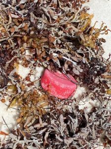
On today’s hike there was quite a bit of this seaweed washed ashore. Most of the marine life living in the seaweed sense the waves and the impending beaching, and jettison for mats further offshore. So, you usually do not find many creatures in the seaweed washed ashore, but sometimes you do. You can take a small dip net out deeper and grab some still floating and you may have better luck. Today, I explored what was washed ashore and did not find much. I did find a lot of plastic, and those who study Sargassum ecology will tell there is a lot of plastic debris caught up in the Sargassum mats. Today I noticed a lot of bottle caps. Not many bottles, but lots of bottle caps. As many others do, we encourage everyone to dispose of the garbage properly. I read this week of a manatee found near Mobile Bay earlier this year who died of cold stress but had swallowed a plastic bag, which was caught in his throat. Marine debris kills. Please dispose of your trash properly.
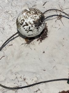
This crab pot float was one of several debris items washed in with the sargassum.
Heading inland to the dune field I heard sirens. The beach patrol was answering a call. I am not sure where, nor what the issue was, but these again are sounds I do not usually hear when hiking early and late in the day. There are currents in the Gulf that can suck you out to sea, and each year we have visitors drown not knowing where these currents are, or how to get out of them if they are caught in one. Pay attention to the colored flags and be careful. I never saw, nor heard, an ambulance follow the beach patrol. So, I am guessing everyone was okay on this call.
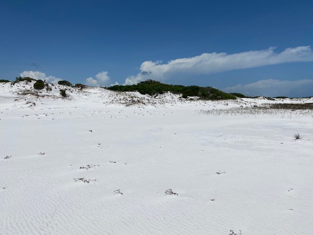
The dune field on this May afternoon was warm. There was a light breeze from the southeast that kept things from getting too warm, but it was warm none the less. As we move closer the hot days of summer the wildlife will move more at dawn and dusk, as well as in the evening. I was not expecting to see a lot on this hike.
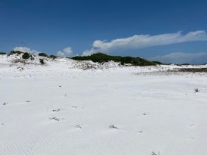
This flat area of the dune field was quite warm on this afternoon and made me think of crossing a desert.
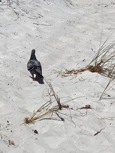
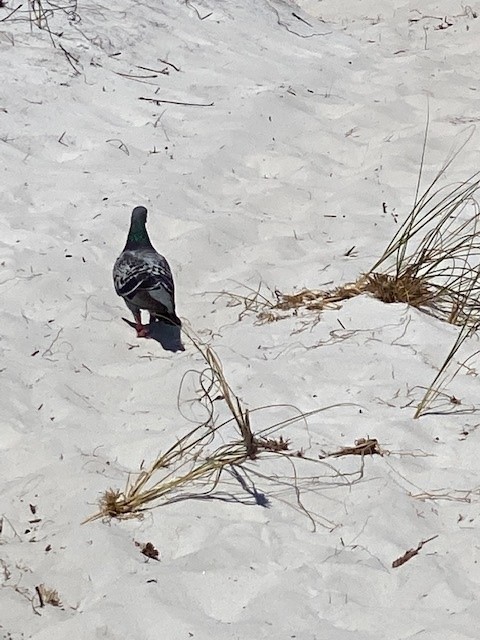
This was an unusual site, a pigeon walking in the open dune field.
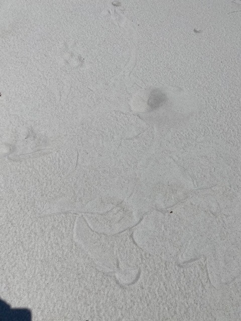
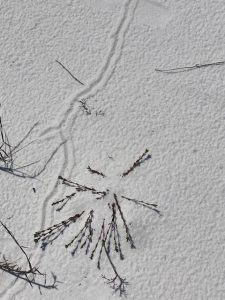
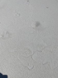
As always you can see what has been moving by searching for tracks and tracks, I did find. Many of them were human, indicating the tourist season is upon us, but there were tracks of animals as well. There were plenty from our friends the raccoon and armadillo. I did notice more raccoon tracks this month. I and my volunteers who survey nesting beaches notice more raccoon tracks this time of year looking for eggs. I also noticed more snake tracks on this hike, they too are mating and moving much more. The lizard tracks were fresh, and I have noticed these moving during the warmer parts of the day and their tracks running across the dune face told me they were very busy that day.
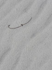
This straight line the sign of a tail drag by a lizard, most likely the six-lined skink.
Many who visit the dunes of our barriers find these burrow looking trails. These are made by beetles.
I followed this snake track until I found this – what appears to be a “tussle” the snake had with a possible prey.
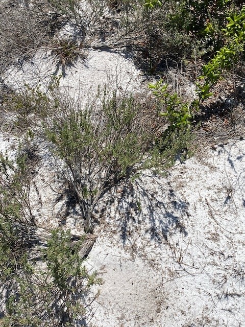
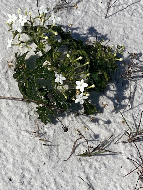
Being spring you would expect flowers, and there were some, just not as many as you might expect. Most of them were white and were blooming on plants near the boggy areas of the swales. The conradina that blooms more in the winter, was done and the blossoms were gone. I did see the early stages of the magnolia flowers trying to come up, but the bright green shoots of new growth on the pines were not visible. There were bees, lots of bees.

The lavender blossoms of the false rosemary, which appeared in winter, are now gone.
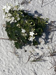
White flowers were common on this spring afternoon. Such as this one on the spiny bull nettle.
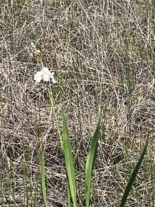
Another white flower is seen on this Sagittaria growing in one of the swales between dunes.
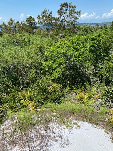
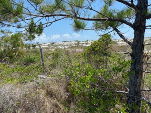
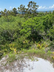
I hiked through a small pine scrub area thinking I might someone in the shade avoiding the heat of the day but did not find anything. I went along the edge of the tertiary dunes where they meet the maritime forest looking for the same thing. Nothing, but there were tracks. The cactus seemed to be more abundant this month.
The pine scrub offered one of the few places with shade.
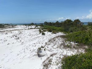
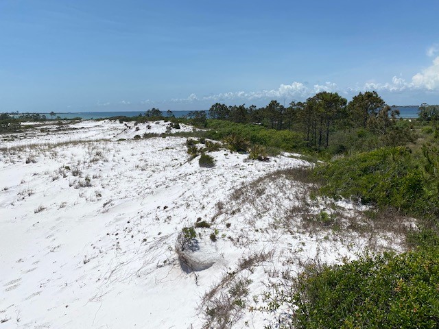
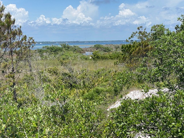
The dune field of a Florida panhandle barrier island.
From atop of one of the higher dunes you can see the steep drop towards the marsh.
Along the ridge between the maritime forest and the salt marsh is where I found the otter slide last month. I did not see any evidence of otters today. The bird action was slower today as well. Maybe because of the heat they too had settled somewhere. I did not see an osprey, which is unusual.
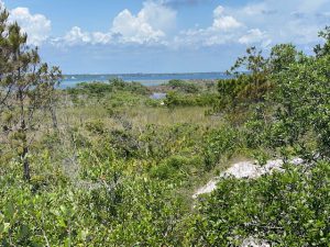
Big Sabine as seen from atop one of the larger dunes.
As I reached the beach of the Sound, I did notice a LOT of digging by armadillos. They had been very active. There were no snakes or marsh rats. There were again people, these were on jet skis. There were a few fishing from small boats. With no rain over the last week or so the visibility in the Sound was amazing, but I only saw one small blue crab. No hermit crabs and not any fish. However, the lagoon of the marsh the killifish, also known as bull minnows, were abundant and the males all aglow with their iridescent blue colors of breeding season. The males were chasing each other all over the tidal pools and open water of the lagoon designating their territories for current breeding that would follow. I did notice more crows than I usually do and what made me catch their attention was the constant calling at me and the hovering over me suggesting they too were breeding, and an active nest was nearby.
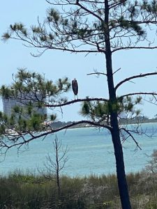
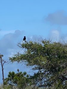
A blue heron is seen sitting in a pine overlooking Santa Rosa Sound.
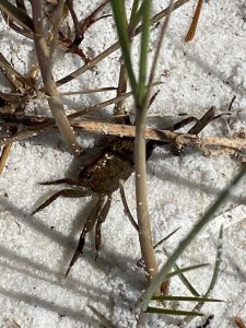
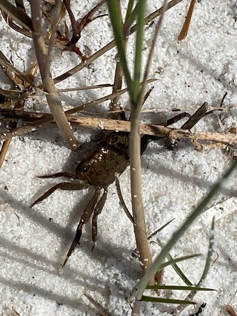
A small Seserma crab is seen hiding under grass along the beach of the Sound.
The crows were numerous and active on this spring afternoon.
I was not expecting much hiking in the middle of the afternoon, but it is always good to do these just to see what is moving. I hope to do another hike this month either early in the morning or late in the afternoon. Maybe we will see more.
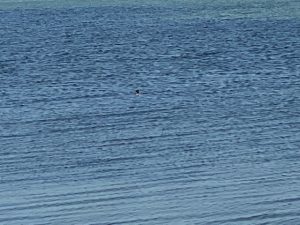
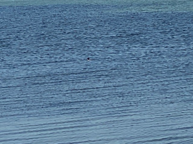
It may be hard to see, but there was a small duck enjoying the Sound.
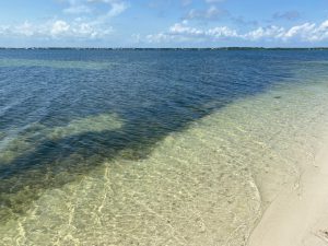
With little rain over the last few days the water clarity was excellent and you could see the seagrass very well.
by Rick O'Connor | May 13, 2022
EDRR Invasive Species
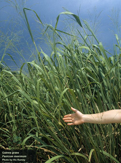
Guinea Grass (Megathyrus maximum)

Guinea Grass
Photo: University of Florida IFAS
Define Invasive Species: must have ALL of the following –
- Is non-native to the area, in our case northwest Florida
- Introduced by humans, whether intentional or accidental
- Causing either an environmental or economic problem, possibly both
Define EDRR Species: Early Detection Rapid Response. These are species that are either –
- Not currently in the area, in our case the Six Rivers CISMA, but a potential threat
- In the area but in small numbers and could be eradicated
Native Range:
Guinea grass is native to Africa.
Introduction:
The plant was introduced as livestock fodder.
EDDMapS currently list 2,614 records of guinea grass. Most records come from Florida and Texas, but it has also been reported in Hawaii and Puerto Rico. In Florida it has been reported across the state. There are 17 records in the Florida panhandle, 15 of those within the Six Rivers CISMA, 12 of those within the CISMA were reported from the Yellow River Preserve area in Santa Rosa County and the remaining three were from Eglin AFB.
Description:
This is a large panicum grass reaching heights of up to seven feet and grows in dense mats. The strap-like blades and smooth and up to three feet long and two inches wide. The seed inflorescence is large as well, reach two feet in length.
Issues and Impacts:
Guinea grass is an aggressive growing plant that will quickly occupy disturbed open spaces and form thick monocultures decreasing native plant abundance and overall biodiversity.
Management:
The recommended management is foliar spraying with a 1% solution of glyphosate. Care should be taken not to overspray because this herbicide is non-selective and will kill other desirable plants.
Please report any sighting to www.EDDMapS.org
For more information on this EDRR species, contact your local extension office.
References
Urochola maximum. Guinea Grass. University of Florida Center for Aquatic and Invasive Species. | Center for Aquatic and Invasive Plants | University of Florida, IFAS (ufl.edu).
Sellers, B., Smith, H., Ferrell J. 2018. Identification and Control of Johnsongrass, Vaseygrass, and Guinea Grass in Pastures. University of Florida Electronic Data Information System. SS-AGR-363. pdf\AG\AG372\AG372-16272415.pdf (ufl.edu)
Early Detection and Distribution Mapping System (EDDMapS)
https://www.eddmaps.org/
Six Rivers CISMA
https://www.floridainvasives.org/sixrivers/
by Rick O'Connor | May 6, 2022
Imperiled (verb) – put at risk of being harmed, injured, or destroyed.
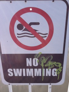
In 2021 the Florida Department of Environmental Protection classified 44 area waterways in the Pensacola Bay System as imperiled. Such designations are based on an environmental parameter making it unhealthy for one reason or another. When we think of an unhealthy body of water, many times we think of sewage. There are nine bodies of water in the Pensacola Bay System classified as imperiled due to the fecal bacteria concentrations within. There are another seven for bacteria levels high enough to close them for shellfish harvesting. This is a total of 16 bodies of water having bacteria issues (36% of the 44 designations).
Closed due to bacteria.
Photo: Rick O’Connor
Low dissolved oxygen and fish kills is another parameter we think of. There are four waterways designated imperiled due to high nutrients (a cause of hypoxia and fish kills), and one for low dissolved oxygen readings itself. This is a total of five (11% of the 44 designations).
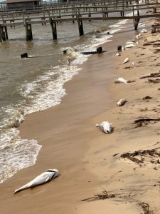
Dead redfish on the eastern shore of Mobile Bay.
Photo: Jimbo Meador
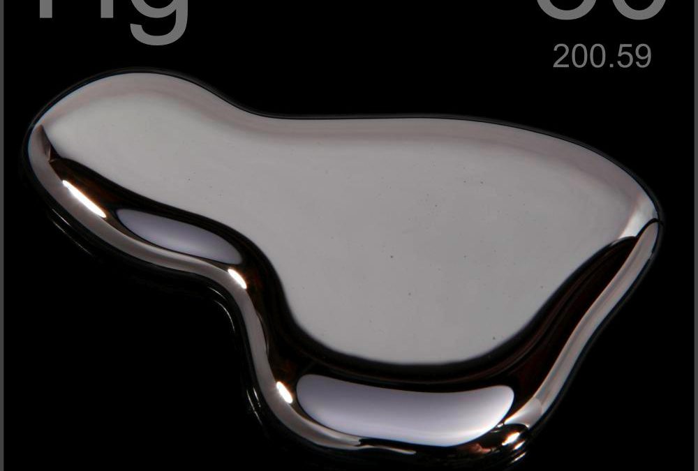
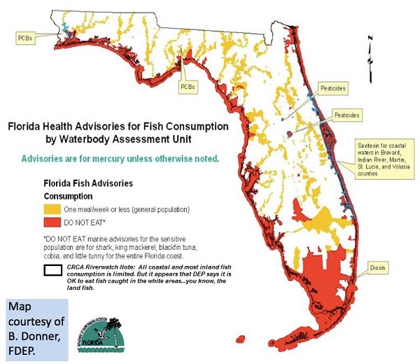
But you may be surprised to learn that 23 of the 44 imperiled water bodies (52%) are designated based on the mercury content of the fish sampled there.
Most people are aware of the mercury issue in fish. Many of those living in the Pensacola Bay area are aware of this issue locally, but they may not be aware that with the 2021 designations, it is the primary reason for many listed. To be fair, it is not that mercury issues are increasing, it may be more that there are 97 waterways in the Pensacola Bay System being considered for delisting in 2021 and those are listed for a variety of other issues. What it is stating is that with the 44 that remain imperiled, mercury is the primary cause.
We have all heard of mercury in fish, but where is it coming from? What health problems does it cause? And is there anything that can be done to make these bodies of water healthier?
Mercury is a naturally occurring element on the periodic table. It is element #80, meaning it has 80 protons and electrons, one of the larger naturally occurring elements. It is a silver-colored liquid at room temperature, one of only two naturally occurring elements in the liquid phase at these temperatures – the other being bromine. It is sporadically found throughout the earth’s crust, usually combined with other elements. There are two forms of mercury – mercury (I) and mercury (II) – indicating the number of cations available for sharing or transferring in compound bonding. Mercury (II) is more common in nature.
The element has been of interest to humans for centuries. There are records of it buried beneath the Mayan pyramids, though we are not sure how it was used, and it was used in Chinese medicine centuries ago. The Spanish used it to help extract silver from mines during their colonial period around the world. It was also used in separating fir from skin in felt hat making in the 19th century. Hatters who used this method eventually had neurological problems and became known as “mad hatters”, an idea used in Lewis Carol’s Alice’s Adventures in Wonderland.
In more modern times it has been used in fillings for tooth cavities (including my own) and preserving specific vaccines. Being a good conductor of electricity and not of heat, it is used in numerous electrical components, fluorescent lighting, and batteries. Some cultures used it to help “whiten their skin” and a common use is in the processing and production of certain industrial chemicals. Today, due to the toxic properties of mercury, many of these uses are no longer.

Fluorescent lighting contains mercury.
Mercury is obtained for these uses by mining their ores. The most sought after ore is cinnabar, a red-colored rock found around the world. Mercury (II) sulflide (HgS) is a common compound found in cinnabar. When heated and oxidized it will produce sulfur dioxide and elemental mercury.
HgS + O2 à Hg + SO2
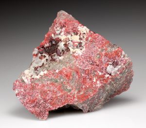
Cinnabar is the most common ore mined for mercury.
Photo: Classic Crystal
The problem with mercury is that it is toxic, and some forms of mercury are more toxic than others. The element is known to cause brain, kidney, and lung issues. It also can weaken the immune system. It is most known for the neurological problems it causes. Sensory impairment, lack of motor skill coordination, psychotic reactions, hallucinations, tremors and spasms have all been connected to exposure to mercury. There are concerns with the neurological development within the fetus if exposed to mercury and many of the health advisories target women of childbearing age who are pregnant or considering it. They have included the very young and the very old in their recommendations that these members of the population do not eat more than 6 ounces of fish (or shellfish) that have high mercury contamination.

Mercury contamination in fish.
Image: BBC
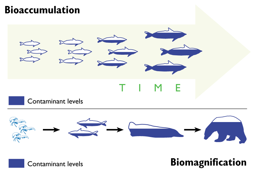
The organic forms of mercury, dimethylmercury and methylmercury, are the more toxic forms. These are introduced to the environment both naturally and from human activity. Once in the aquatic environment they are absorbed by the phytoplankton (microscopic plants in aquatic environments). Methylmercury accumulates in lipids (fats) within the cell at relatively low concentrations (phytoplankton are not large). However, they are not passed by the creature. The slightly larger zooplankton (microscopic animals) feed on the phytoplankton and accumulate the mercury they have stored. Feeding on a lot of these, they accumulate even more mercury. The zooplankton are consumed by small fish, who eat a lot and accumulate even more mercury. Then the mid-sized fish consume them, and the larger fish consume those, and on and on. The top predators have accumulated enough methylmercury to be hazardous to human health IF they are consumed by people. This process of increasing the concentration of mercury through the food chain is known as biomagnification – “magnifying the problem”.
So, which fish are of concern?
Based on the Florida Department of Health for freshwater systems in Escambia County.
- Bluegill, Channel catfish, Largemouth bass, Long-eared sunfish, Red-eared sunfish, Spotted sunfish and Warmouth from the Escambia River system – you should not eat more than one/week.
- Do not eat chain pickerel or largemouth bass – and do not consume more than two red-eared sunfish from Crescent Lake.
- Lake Stone near Century FL – no more than two bluegill and sunfish per week and no more than one largemouth bass each week.
- From the Perdido River do not eat more than two bluegill or sunfish each week and do not eat largemouth bass from the Perdido River.
- The same species and regulations apply for the Yellow River system as well.
The following marine species are of concern….
Almaco jack, Atlantic spadefish, Atlantic croaker, Weakfish (trout), Black drum, Black grouper, Blackfin tuna, Bluefish, Cobia, Dolphin, Pompano, Gafftop catfish, Gag, Greater amberjack, Gulf flounder, Hardhead catfish, King mackerel, Ladyfish, Lane snapper, Bonito, Mutton snapper, Pigfish, Red grouper, Red snapper, Sand seatrout, Scamp, Shark, Sheepshead, Snowy grouper, Southern flounder, Southern kingfish, Spanish mackerel, Spot, Striped mullet, Vermillion snapper, Wahoo, White mullet, Yellow-edge grouper, and Yellowfin tuna.
In each case it is not recommended eating more than two servings a week. For a few, it is recommended that the most vulnerable people mentioned earlier not at ANY… Those would include Blackfin tuna, Cobia, King mackerel, Bonito, and Shark.
It is recommended that NO ONE eat king mackerel over 31 inches and any shark species over 43 inches in length.
I guess as you look at this list, you see fish species that you like. This list can lead folks to think… “I am just not going to eat seafood”. This would be a mistake. The Department of Health has found there are essential vitamins and nutrients provided be seafood that are missing if you do not eat them. They found additional problems in fetal development when seafood protein was left out of the mothers’ diet. So, the response would be… eat other seafood species you do not see on this list… or, if you see something you do like, no more than 1-2 6-ounce servings per week.
So, is there anything we can do about the mercury issue in our bay system?
Well, to have the biggest impact you will need to determine the biggest source. 33% of the mercury in our environment comes from natural sources, such as volcanic eruptions. We can do nothing about volcanic eruptions, or other natural sources, so we will need to look at anthropogenic (human) sources.
The larger sources would be anthropogenic, which account for 67% of the known mercury in the environment, focusing on these can make a large impact. Coming in at No.1 – producing electricity by burning coal. This accounts for 65% of the anthropogenic sources. Moving away from burning coal would make a huge difference. But that is easier said than done. Mining and burning coal are important for the economy of many communities. It is one of the cheaper methods of producing much needed electricity. But in addition to producing mercury compounds during the heating process, many other toxic compounds are produced and released as well – not to mention the amount of greenhouse gases produced during this process. Hence the name “dirty coal”. There are other methods of producing electricity and the solution would be to convert not only the power plants to these methods, but the coal dependent communities to this line of work. This one step would make a big difference.
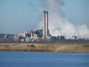
Power plant on one of the panhandle estuaries.
Photo: Flickr
At a much smaller scale, mining for gold produces 11% of the mercury from the mine tailings, cement production (7%), and incinerating garbage (3%). Though not a large player in this game, reducing the amount of solid waste burned each year would help reduce the mercury issue.
The takeaway here is that the number of imperiled waterways in the Pensacola Bay System have been reduced over recent years and we will look at this in another article. But for those that remain, mercury is the prime reason. It is also important to understand that mercury is a naturally occurring element and can not be broken down, so we have what we have – but, we can stop adding to the problem. Third, eating some seafood each week is good for you. You will just need to select species that are not problems or watch how much you eat if you prefer some of the listed species.
For more information on the 2021 imperiled waterways list visit
https://floridadep.gov/dear/watershed-assessment-section/content/final-lists-impaired-waters-group-4-cycle-2-basins
For more on the seafood safety species lists visit
https://dchpexternalapps.doh.state.fl.us/fishadvisory/
Other sources for this article included:
Wikipedia – https://en.wikipedia.org/wiki/Mercury_(element)
Miller, G.T., Spoolman, S.E. 2011. Living in the Environment. Brooks and Cole Cengage Learning. Belmont CA. pp. 674.